This is the manual for pplacer, which places query sequences on a fixed reference phylogenetic tree according to a reference alignment. Pplacer was written by Frederick "Erick" Matsen, with very valuable input from Robin Kodner and Ginger Armburst. Special thanks go to Chris Berthiaume and David Schruth at the Armburst lab.
- Contents
- Introduction
- How to avoid reading this manual
- Running pplacer
- What is "playing baseball?"
- About the EDPL metric
- Visualizing the results using placeviz
- Combining and splitting results using placeutil
- Format of the place file
- Making trees for use with pplacer
- Alignment and searching
- A complete example
Introduction
Pplacer places query sequences on a fixed reference phylogenetic tree according to a reference alignment. In maximum likelihood (ML) mode, pplacer tries to find the attachement location and the pendant branch length which maximize the likelihood of the tree with pendant branch length attached. In Bayesian posterior probability (PP) mode, pplacer tries to find the edge attachment which maximizes the posterior probability of a fragment placement on an edge conditioned on the reference tree (with branch lengths).
The pplacer suite of programs currently consists of three executables, all of which are described here:- - pplacer, which takes reference information and query sequences and places the query sequences onto the fixed reference tree
- - placeviz, which makes visualizations in phyloXML and Newick format out of the pplacer output
- - placeutil, which combines and splits apart collections of placements.
How to avoid reading this manual
If you've read the paper and know what's going on, look at the example runs, and have a look at how to make trees for use with pplacer. Another important point is that your query sequences need to be aligned to the fixed reference alignment. This is addressed in more detail in the alignment section. Then you can follow along the example with your data. Once you have run pplacer and have some .place files in hand you can go back and look at what to do with them.Running pplacer
Pplacer requires a reference alignment, a reference tree, and the ML parameters for that reference tree. In principle these can be made with any ML phylogenetics implementation, but pplacer works real slick with phyml version 3 and RAxML. Both of these packages return an optimal tree as well as a file containing the ML parameters for the tree model, things such as the gamma shape parameter, and the GTR rate parameters if one is using that model. We will call this ML parameter file the "statistics" file.
A basic pplacer runs looks like
pplacer -r reference_alignment -t reference_tree -s statistics_file queries.fastafor a ML run, and
pplacer -p -r reference_alignment -t reference_tree -s statistics_file queries.fasta
for a ML + Bayes run (-p signifies posterior probability).
As usual, you can specify -r, -t, and -s in any order. You can run pplacer with trees made from any ML phylogenetics software, but you will have to specify parameters via the command line, and may have to put together your own statistics file to specify rate parameters. [Note that spaces are not allowed in any file names!]
The query sequences must be in FASTA file format. The reference alignment can be in FASTA or non-interleaved phylip format.
It's not a bad idea to keep all of your reference alignments and trees for a given alignment distinct from the pplacer run. That way, you can just have a single copy of all of the reference information, which ensures that it's the same for all of your query data sets. To enable that type of organization, pplacer has a -d flag which sets the directory for the reference information. It's used like so:
pplacer -d /my/favorite/alignment/dir -r reference_alignment -t reference_tree -s statist...
That way, pplacer looks for reference_alignment, reference_tree, etc in the directory /my/favorite/alignment/dir. Note that it will still read query sequences from the current working directory. It will also write to the current working directory unless otherwise specified by invoking --outDir.
Running pplacer with a phyml v3.0 tree
Phyml's output trees end with "phyml_tree.txt" and its statistics files end with "phyml_stats.txt". Thus a pplacer run using a phyml tree looks likepplacer -r test.fasta -t test.phy_phyml_tree.txt -s test.phy_phyml_stats.txt queries.fasta
Running pplacer with a RAxML tree
RAxML's output trees start with "RAxML_result" and its statistics files start with "RAxML_info". Thus a pplacer run using a RAxML tree looks likepplacer -r test.fasta -t RAxML_result.test -s RAxML_info.test queries.fasta
In any case, the result from running pplacer is to get a place file. This file contains information about where the query sequences fit in the tree. This file is human readable, and is described here. However, most folks will want to visualize the placements using placeviz, described here.
pretending
Sometimes you want to check if your input data looks OK before actually running an analysis. For that pplacer supplies a --pretend option, run like so:pplacer --pretend -r test.fasta -t RAxML_result.test -s RAxML_info.test queries.fasta
It just checks the basics, so if you try to sneak past it I'm sure that you can.
What is "playing baseball?"
If you are watching pplacer run, you will see the following messages:
Running pplacer analysis...
Caching likelihood information on reference tree... done.
Preparing the edges for baseball... done.
Baseball? "Playing baseball" is one way that pplacer substantially increases the speed of placement, especially on very large trees. Baseball is a game where the player with the bat has a certain number of unsuccessful attempts, called "strikes", to hit the ball.
Pplacer applies this logic as follows. Before placing placements, the algorithm gathers some extra information at each edge which makes it very fast to do a quick initial evaluation of those edges. This initial evaluation of the edges gives the order with which those edges are evaluated in a more complete sense. We will call full evaluations "pitches." We start with the edge that looks best from the initial evaluation; say that the ML attachment to that edge for a given query has log likelihood L. Fix some positive number D, which we call the "strike box." We proceed down the list in order until we encounter the first placement which has log likelihood less than L - D, which we call a "strike." Continue, allowing some number of strikes, until we stop doing detailed evaluation of what are most likely rather poor parts of the tree.
You can control the behavior of baseball playing using the --maxStrikes, --strikeBox, and --maxPitches options. If, for any reason, you wish to disable baseball playing, simply add --maxStrikes to zero (this also disables the --maxPitches option).
Having control over these options raises the question of how to set them. The answer to this question can be given by pplacer's "fantasy baseball" feature. To gain an understanding of the tradeoff between runtime and accuracy, it analyzes all --maxPitches best locations. It then runs the baseball algorithm with each combination of strike box (from 0 to the specified --strikeBox) and max strikes (from 1 to the specified --maxStrikes). Using these different settings the program reports
- - the "batting average," i.e. the number of times the baseball algorithm with those settings achieved the optimal location obtained by evaluating all --maxPitches best locations; found in the file prefix.batting_avg.out
- - the "log likelihood difference," i.e. the difference between the ML log likelihood achieved by the baseball algorithm with those settings compared to the best obtained by evaluating all --maxPitches best locations; found in the file prefix.like_diff.out
- - the "number of trials," i.e. the number of locations fully evaluated by the baseball algorithm with those settings; found in the file prefix.n_trials.out
pplacer --maxStrikes 10 --strikeBox 10 --fantasy 0.05 --fantasyFrac 0.02 -r example.fasta...
says to run pplacer trying all of the combinations of max strikes and strike box up to 10, looking for the optimal combination which will give an average log likelihood difference of 0.05, and running on 2% of the query sequences. If, for any reason, you wish to disable baseball playing, simply add --maxStrikes to zero (this also disables the --maxPitches option).
You can use R to plot these matrices in a heat-map like fashion like so:
ba <- read.table("reads_nodups.batting_avg.out")
image(x=c(0:nrow(ba)-1),xlab= "strike box", ylab= "number of strikes", \
   y=c(1:ncol(ba)-1),z=as.matrix(ba), main="batting average")
About the EDPL metric
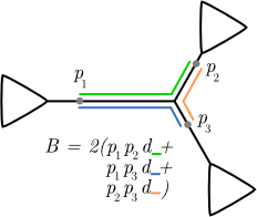
The expected distance between placement locations (EDPL) is a means of understanding the uncertainty of a placement using pplacer. The motivation for using such a metric comes from when there are a number of closely-related sequences present in the reference alignment. In this case, there may be considerable uncertainty about which edge is best as measured by posterior probability or likelihood weight ratio. However, the actual uncertainty as to the best region of the tree for that query sequence may be quite small. For instance, we may have a number of very similar subspecies of a given species in the alignment, and although it may not be possible to be sure to match a given query to a subspecies, one might be quite sure that it is one of them.
The EDPL metric is one way of resolving this problem by considering the distances between the possible placements for a given query. It works as follows. Say the query bounces around to the different placement positions according to their posterior probability; i.e. the query lands with location one with probability p1, location two with probability p2, and so on. Then the EDPL value is simply the expected distance it will travel in one of those bounces (if you don't like probabilistic language, it's simply the average distance it will travel per bounce when allowed to bounce between the placements for a long time with their assigned probabilities). Here's an example, with three hypothetical locations for a given query sequence:
Visualizing pplacer results using placeviz
Placeviz is a utility for visualizing place files. It is available for OS X, so you can download a place file from a cluster to your macinblock and look at it there. It's easy to use:
placeviz example.placeThe default is to use the maximum likelihood values for visualizations, which will make files with the "ML" infix, such as example.ML.fat.xml. If you ran pplacer with the -p option and want to use the posterior probabilities for assignment, then just run pplacer with the -p option.
placeviz -p example.placeThis will make files with the "PP" infix. Placeviz writes out visualizations in phyloXML format, as well as the more common Newick format.
visualizations using phyloXML format
These visualizations can be viewed using Christian Zmasek's archaeopteryx software. To show branch widths and colors, not that you must download the archaeopteryx configuration file and put that file in the same directory as the forester.jar application.
.fat.xml
This tree makes the reference tree have branch widths equal to a linear function of the number of placements assigned to that edge. Here's an example of a portion of such a tree:
The amount of width per placement is determined by using one of two options, either --unit-width, which specifies the number of pixels per placement (usually a number less than one!) or --total-width, which specifies the total number of pixels used for phylogenetic placements.
.edpl.xml
This makes a fat tree which is colored according to the EDPL uncertainty, and same width options apply as for the fat tree above. The argument to --edpl gives the EDPL level which will correspond to 100% red; any branches with average EDPL above that level will show up as yellow. Here's an example of a portion of such a tree:
The --whitebg option makes colors which are more appropriate for a white background (including for export to PDF). You can see an example of this sort of visualization on the visualization page.
visualizations using Newick format
.tog.tre
With the --tog option, it makes a .tog.tre file showing the placements (highlighted in red using FigTree) in their ML location with their ML branch lengths on the tree. That can get a bit busy with many thousands of placements, so we also have the .num.tre mode described next.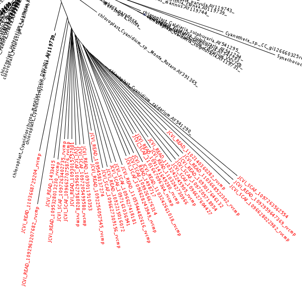
.num.tre
The .num.tre file simply summarizes the number of placements on a given edge with X_at_Y, saying that there were X placements at the edge numbered Y. The corresponding sequences can be found in the .loc.fasta file as described above.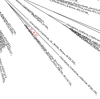
.loc.fasta
With the --loc option, it makes a .loc.fasta file is a fasta file which has been organized according to placement location. The different locations are separated by dummy sequences whose names describe the various locations. One can look at this file using any multiple alignment viewer to get an idea of the clustering of various sequences. This is a screenshot from geneious (note that the screenshot cuts off the majority of the alignment.)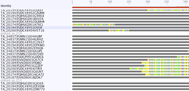
Combining and splitting results using placeutil
Placeutil is a utility which helps organize pplacer results. It can split up and recombine place files as we will see.
The following combines ex1.place and ex2.place into a single file, combo.place, sorted according to placement location:
placeutil -o combo ex1.place ex2.place
This can be used for combining results from parallelized runs.
We can then split up the placements based on EDPL or likelihood weight ratio, like so:
placeutil --edpl -c 0.01 combo.place
This makes two files, combo.ML.edpl.ge0.01.place and combo.ML.edpl.lt0.01.place. The file combo.ML.edpl.ge0.01.place contains those placements with ML EDPL ratio greater than or equal to 0.01, and combo.ML.edpl.lt0.01.place contains the rest.
We can also split up the placements based on name matching. That way one can combine samples from multiple data sets into a single pplacer run, then separate later based on different conditions or sample sites. The names are split based on regular expressions, specifically the implementation here. It's not as fun as using PCRE or the python re module, but it should suffice. To split in this way, make a file with the desired prefix then the regular expression in quotes (comment lines beginning with # are ignored). For example, we could put
set_1  "^R1_"
set_2  "^R2_"
in a file called "sepfile.txt." Then
placeutil --reSepFile sepfile.txt combo.place
separates combo.place into two files, set_1.place (containing all of the queries whose names begin with "R1_") and set_2.place (containing all of the queries whose names begin with "R2_").
Format of the place file
The place file contains the output of a pplacer run. It is self contained, containing all of the information specified except for the reference alignment. We'll just take a quick look here.
The file starts with some information about how pplacer was run. These lines start with #. It is very important not to modify this information (especially the reference tree) by hand, or else the correct location of the placements will be lost.
After those lines come the placements. The format is fasta-like. First comes the name of the query sequence, then the query sequence, then lines describing the places where that sequence seems to fit. The entries are ordered as follows:
- Placement edge number, numbered as in a postorder traversal
- ML likelihood weight ratio (i.e. the normalized ML likelihood values)
- Posterior probability (or a dash if the -p option was not set)
- ML log likelihood
- Bayes marginal likelihood (or a dash if the -p option was not set)
- The ML distance from the distal (farthest from the root) side of the edge
- The ML pendant branch length
Note that the likelihoods given are the product of the site likelihoods for sites which are known and not gapped in the query sequence. We only need to calculate those likelihoods because in the end we are primarily interested in ratios of them, and the unknown/gapped sites will cancel out in that ratio. Therefore we can only compare those likelihoods to traditional phylogenetics implementations when there are no gaps in the query sequences. I've compared to phyml, and yes, they do give the same values.
For example is the result for a single query, J1fw_FTWCYXX01AH60X.
>J1fw_FTWCYXX01AH60X
????????????????????????????GGCAGTCTAGCAGAAGAAAGAGTAATAATTAGATCTCAAAATATCACAAATAA...
10   0.799166   0.747362   -7980.32   -7982.81   0.0953686    0.117152
11   0.137794   0.143586   -7982.08   -7984.46   0.00567305   0.0963186
Pplacer liked two edges in the tree, 10 and 11, for the query sequence. To see where that is, one could stare at the numbered reference tree, but it's probably best to use placeviz.
To edge 10, it attached a likelihood weight ratio of 0.799166, and a posterior probability of 0.747362. The likelihood was -7980.32 and Bayes marginal likelihood of -7982.81. The ML attachment location along edge 10 was 0.0953686 from the distal (farthest from the root) side of the edge, and ML pendant branch length was 0.117152.
Making trees for use with pplacer
Phyml and RAxML are two nice packages for making ML trees that we have used extensively. Phyml has a nice webserver, but RAxML is the choice for very large trees. Pplacer only knows about the GTR, WAG and LG models, so use those to build your trees. If you are very fond of another model and can convince me that I should implement it, I will.
Both of these packages implement gamma rate variation among sites, which accomodates that some regions evolve more quickly than others. That's generally a good thing, but if you have millions of query sequences, you might have to run pplacer with fewer rate parameters to make it faster.
I run phyml like so, on non-interleaved (hence the -q) phylip-format alignments:
phyml -q -d nt -m GTR -i nucleotides.phy
phyml -q -d aa -m WAG -i amino_acids.phy
Note that pplacer only works with phyml version 3.0 (the current version).
I run RAxML like so, on similar alignments (the "F" suffix on PROTGAMMAWAGF means to use the emperical amino acid frequencies):
raxmlHPC -m GTRGAMMA -n test -s nucleotides.phy
raxmlHPC -m PROTGAMMAWAGF -n test -s amino_acids.phy
Even though Alexandros Stamatakis is quite fond of the "CAT" models and they accelerate tree inference, they aren't appropriate for use with pplacer. We need to get an estimate of the gamma shape parameter.
If your taxon names have too many funny symbols, pplacer will get confused. We have had a difficult time with the wacky names exported by the otherwise lovely software geneious. If you have a tree which isn't getting parsed properly by pplacer, and you think it should be, send it to me and I'll try to have a look.
At least for now, we do not recommend that you give pplacer a reference tree with lots of very similar sequences. It's certainly a bit of a waste of time-- pplacer must evaluate the resultant branches like any others. But worse, it can foul up the analysis. If one has a clade of very similar sequences, a query sequence which is similar to those sequences can fit anywhere in the clade. The resulting uncertainty will then be reported as a low ML ratio or posterior probability, even if pplacer is quite confident that the query fits in that clade. Pplacer also has computational difficulty with exceedingly short ("zero") length edges. We are currently considering ways to work around these issues.
If you give pplacer a reference tree which has been rooted, you will get a warning like
Warning: pplacer results make the most sense when the given tree is multifurcating at the
root. See manual for details.
In pplacer the two edges coming off of the root have the same status as the rest of the edges; therefore they are be artifically counted as two separate edges. That will lead to artifactually low likelihood weight ratio and posterior probabilities for query sequences placed on those edges. This doesn't matter if your query sequences do not get placed next to the root, but you can avoid the problem altogether by rooting the tree at an internal node, or by leaving the outgroup in and rerooting the placeviz trees.
Alignment and searching
The alignment situation for pplacer differs a bit than for other phylogenetic packages. Pplacer is just comparing the sequence information in the fragment to the reference alignment, therefore a complete multiple alignment with all however-many-reads is thankfully unnecessary. Furthermore, it is crucial that the reference alignment not change in the alignment step. Both of these facts mean that alignment to a profile HMM, as with HMMER, is an excellent choice. HMMER's hmmsearch program can be used to quickly search very large databases of reads for ones that are relevant for the reference alignment of interest, eliminating the need for BLAST.
However, some care needs to be taken in using HMMER for aligning reads for pplacer. We build our HMM with hmmbuild --hand using a RF annotation line which includes everything we want to keep as a consensus column marked with an "x" (see the HMMER manual). Take care doing this: marking "gappy" columns as consensus will defeat HMMER's algorithms for building useful HMMs. Then we use hmmalign --mapali to get an alignment of the fragments with the reference alignment and split the alignment back into the reference and fragment alignment.
A complete example
Here we'll go through a fairly complete example of using pplacer. The Turnbaugh et. al. twins gut study.
The first step is to make a reference tree. Here we do so with RAxML.
raxmlHPC -m GTRGAMMA -n ref_tree -s ref_aln.phy
RAxML makes a number of files; we need RAxML_info.ref_tree, the "statistics" file, and RAxML_result.ref_tree, the final tree file.
Now we are ready to actually run pplacer.
pplacer -d refs \
	-t RAxML_result.ref_tree \
	-r ref_aln.fasta \
	-s RAxML_info.ref_tree \
	gut.fasta
As usual, -d specified the directory with the reference information, -r the reference alignment, -t the reference tree, and -s the statistics file. The actual reads come at the end. Note that you don't have to use the backslashes ("\"); we use them here because we wanted to break the command over multiple lines. If we had wanted to compute posterior probabilities, we would have added the -p option.
Upon running this command, pplacer outputs
Running pplacer v1.0.r018 analysis...
refs/RAxML_info.ref_tree
Caching likelihood information on reference tree... done.
Pulling exponents... done.
Preparing the edges for baseball... done.
Finding friends. Read alignment. This will require around 4.995e+05 sequence comparisons... done.
running 'seq0011368' 1 / 1000 ...
running 'seq0005394' 2 / 1000 ...
...
running 'seq0013738' 998 / 1000 ...
running 'seq0006998' 999 / 1000 ...
running 'seq0007013' 1000 / 1000 ...
elapsed time: 00:01:56.7 (116.699 s)
number of garbage compactions: 4
Now we can visualize the results using placeviz:
placeviz *placemaking trees as described in the placeviz section.
That's it! I hope you enjoy using pplacer, and don't hesitate to email me with any comments, problems or questions.