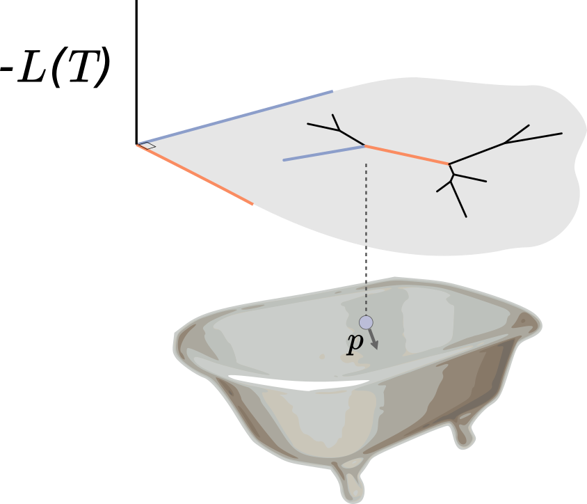
Hamiltonian Monte Carlo (HMC) is an exciting approach for sampling Bayesian posterior distributions. HMC is distinguished from typical MCMC because proposals are derived such that acceptance probability is very high, even though proposals can be distant from the starting state. These lovely proposals come from approximating the path of a particle moving without friction on the posterior surface.

Indeed, the situation is analogous to a bar of soap sliding around a bathtub, where in this case the bathtub is the posterior surface flipped upside down. When the soap hits an incline, i.e. a region of bad posterior, it slows down and heads back in another direction. We give the soap some random momentum to start with, let it slide around for some period, and where it is at the end of this period is our proposal. Calculating these proposals requires integrating out the soap dynamics, which is done by numerically integrating physics equations (hence the Hamiltonian in HMC). The acceptance ratio is determined only by how well our numerical integration performs: better numerical integration means a higher acceptance probability.

Vu had been noodling around with phylogenetic HMC when we heard that Arman Bilge (at that time in Auckland) had an implementation as well. These implementations not only moved through branch length space according to usual HMC, but also moved between topologies. They did this as follows: once a branch length hits zero, leading to four branches joined at a single node, one can regroup those branches together randomly in another configuration and continue. (If you are a phylogenetics person, this is a random nearest-neighbor interchange around the zero length branch.) This randomness, which is rather different than the deterministic paths of classical HMC once a momentum is drawn, is why we call the algorithm Probabilistic Path Hamiltonian Monte Carlo (PPHMC).

The primary challenge in theoretical development is that the PPHMC paths are no longer deterministic. Thus concepts such as reversibility and volume preservation, which are typical components of correctness proofs for HMC, need to be generalized to probabilistic equivalents. Vu had to work pretty hard to develop these elements and show that they led to ergodicity.

On the implementation front, Arman was also working hard to build an efficient sampler. However, the HMC integrator had difficulty going from one tree topology to another without incurring substantial error. We thrashed around for a while trying to improve things with a “careful” integrator that would find the crossing time and perhaps re-calculate gradients at that time, but proving that such a method would work seemed very hard.

Then, magically, our newest postdoc Cheng Zhang showed up and saved us with a smoothing surrogate function. This surrogate exchanges the discontinuity in the derivative for discontinuity in the potential energy, but we can deal with that using a “refraction” method introduced by Afshar and Domke in 2015. This approach allows us to maintain a low error, and thus make very long trajectories with a high acceptance rate.

I’m happy to announce that our manuscript has been accepted to the 2017 International Conference on Machine Learning. Practically speaking, this work is definitely a proof of concept. We have taken an algorithm that was previously only defined for smooth spaces and extended it to orthant complexes, which are basically Euclidean spaces with boundary glued along those boundaries in intricate ways. Our implementation is not fully optimized, but even if it was I’m not sure that it would out-compete good old MCMC for phylogenetics without some additional tricks.

To know if this flavor of sampler is going to be useful, we really need to better understand what I call the local to global question in phylogenetics. That is, to what extent does local information tell us about where to modify the tree? This is straightforward for posteriors on Euclidean spaces: the gradient points us towards a maximum. But for trees, does the gradient (local information) tell us anything about what parts of the tree should be modified (global information)? We’ll be thinking about this a lot in the coming months!